Power Calculations in Stata

NOTE: this article is only a template. Please add content!

add introductory 1-2 sentences here

Read First

• include here key points you want to make sure all readers understand

Guidelines

What data do I need?

You must have:

• Mean and variance for outcome variable for your population
  • Typically can assume mean and SD are the same for treatment and control groups if randomized

• Sample size (assuming you are calculating MDES (δ))
  • If individual randomization, number of people/units (n)
  • If clustered, number of clusters (k), number of units per cluster (m), intracluster correlation (ICC, ρ) and ideally, variation of cluster size

• The following standard conventions
  • Significance level (α) = 0.05
  • Power = 0.80 (i.e. probability of type II error (β) = 0.20

Ideally, you will also have:

• Baseline correlation of outcome with covariates
  • Covariates (individual and/or cluster level) reduce the residual variance of the outcome variable, leading to lower required sample sizes
    • Reducing individual level residual variance is akin to increasing # obs per cluster (bigger effect if ICC low)
    • Reducing cluster level residual variance is akin to increasing # of clusters (bigger effect if ICC and m high)
  • If you have baseline data, this is easy to obtain
    • Including baseline autocorrelation will improve power (keep only time invariant portion of variance)

• Number of follow-up surveys

• Autocorrelation of outcome between FUP rounds

How do I get this data?

You will basically never have the data you need for your exact population of interest at the time when you first do power calculations.

You will need to use the best available data to estimate values for each parameter. Sources to consider:

• High-quality nationally representative survey (e.g. LSMS)
• Data from DIME IE in same country (or region, if pressed)
• Review the literature – especially published papers on the sector and country. What kind of effects? Summary stats available?

If you can’t come up with a specific value you feel very confident in, run a few different power calculations with alternate assumptions and create bounded estimates.

Stata Command Options

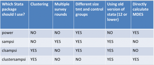
Quick Reference on options:

power

Stata’s newest updated to power calculations. Introduced with Stata13, replaces sampsi.

Pros

• More flexible in terms of input/output choices
• Better output: more info, graph option
• Automatically saves output to a file
• Can compute sample size of control group given treatment group size (or vice versa)
• Directly calculate MDES

Cons

• Doesn’t allow for clustering
• No straightforward way to control for repeated measures
• Allows for treatment and control groups of different sizes

When to use? Simple randomizations (no clustering)

Useful options

• power onemean – assume means same in tmt & control
• n sample size
• n1() control group size, n2() treatment group size
• nratio ratio of n1/n2, default is 1 (not necessary to specify if you list n1 and n2)
• power, table outputs results in table format
• power, saving(filename, [replace]) saves results in .dta format

sampsi

No longer an officially supported stata package (replaced by power), though it continues to work.

Pros

• Works with Stata13 or earlier
• Allows repeated measures (multiple follow-ups)

Cons

• Does not allow clustering
• Have to impute MDES
• Defaults to 90% power (not really a con, but be aware)

Useful Options

• onesample: use if randomized (assume means the same between treatment and control)
• Sample size
  • n1(#) size of treatment group
  • n2(#) size of control group
  • ratio() n1/n2, default is 1
• Repeated measures
  • pre number of baseline measurements
  • post number of follow-up measurements
  • r0(#) correlation between baseline measures (default r0 = r1)
  • r1(#) correlation between follow-up measures
  • r01(#) correlation between baseline and follow-up
• method(post change anova or all), default is all

Back to Parent

This article is part of the topic Sampling & Power Calculations

Additional Resources

• list here other articles related to this topic, with a brief description and link