Event Study

Read First

An event study is a statistical method to assess the impact of an event on an outcome of interest. It can be used as a descriptive tool to describe the dynamic of the outcome of interest before and after the event or in combination regression discontinuity techniques around the time of the event to evaluate its impact. This method has been used mainly in finance to study the impact of specific events on firms value, as it relies on having high frequency data.

Guidelines

As a descriptive tool

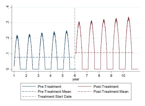
Graphically, an event study will represent one or more time series before and after the event. For example, if we study the impact of an intervention giving improved seeds and cattle to farmers, we can plot the observed value of NDVI (a measure of the growth of plants) on a plot before and after the intervention as below.

In the case above, comparing the average of the poor and after period would, given sufficient power, reject the hypothesis that the average of the outcome variable (in this case NDVI) before the start of the treatment is lower than the average after the treatment begins. This can be a useful tool for exploring hypothesis about whether a program is having an effect.

Without additional structure, however, the difference in means from pre-intervention to post-intervention is NOT a causally valid estimate of the treatment effect, since factors influencing the outcome variable other than the treatment confound the effect. For example, if the landscape is becoming more green for reasons other than fertilizer such as trending changes in temperature, higher NDVI after the distribution of seeds than before distribution can not be causally attributed to the seed distribution.

Treatment effects as deviations from expected trends

Interpreting the differences between post-intervention average and pre-intervention average to the causal effect of a program requires knowing what the average of the post-intervention outcome would have been if the program had not started.

For example, if we assume that exposure to a program has a constant, additive effect on NDVI, then we can rewrite the observed value of NDVI on a given plot as:

NDVI = N + D*Post

where N what the value of NDVI would have been if the program had not started and post is a dummy variable for whether an observation is . If it were possible to know the true value of N, then the causal effect of the treatment would be:

D = E(NDVI - N | Post=1)

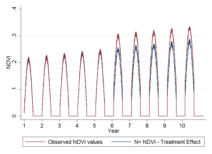
In the picture below, red lines show how NDVI evolves over time (NDVI), while blue lines show how it would have evolved without the intervention starting in year 6 (N). The average treatment effect is the average distance between the red and blue lines in the post-intervention years.

The problem in practice with recovering D is that we do not observe N. So the causal identification problem in event studies is to obtain an estimate of N, N_hat, such that:

E(NDVI-N_hat) = E(NDVI-N)

The interpretation of N_hat is the predicted value of NDVI. Causal identification of treatment in event studies rests entirely on the strength of prediction of N_hat. Any errors in prediction that are correlated with treatment status will confound the estimated treatment effect.

Identifying a casual estimate of the treatment effect in event study, rises or falls on the strength of the prediction of N_hat. When data is available on people or places not exposed to a program N_hat can be estimated from the dynamics of NDVI in non-treated areas. For example, differences-in-differences is a method to estimate N_hat as the average of NDVI in non-treated areas.

In pure event study designs, untreated units are either not available or cannot be used because of selection bias. In such a case, estimates of N_hat come the observation that prior to the start of the program it is by definition true that:

NDVI = N

This identity allows us to estimate N from observable characteristics that could be associated with N. A simple estimate of N from observable characteristics X comes from a regression of N on X as follows:

(NDVI | Post=0) = a + B*X + e

We can therefore find an estimate of B via OLS as by regressing NDVI on observables. With an estimate of B in hand, B_hat, we can form a prediction of D as:

D = E[(NDVI | Post==1) - B_hat*X]

where X is the vector of observable characteristics of plots measured after the introduction of treatment. D will be a valid estimate of treatment effects if two assumptions hold: 1. All characteristics that are correlated with both NDVI and treatment are included in the vector X and 2. The relationship between X in NDVI is the same in the pre-treatment period as in the post-treatment period. These are both very strong assumptions in practice. They are unlikely to be met with sparse data from the pre-intervention period or in cases where the post-intervention context is very different from the pre-intervention context. One method of satisfying the demand for similarity of pre- and post- period constraint is to use techniques of regression discontinuity around the date in which treatment begins.

The increasing availability of large, high frequency datasets are improving the potential of estimating N_hat through machine learning approaches. [1]

Regression Discontinuity

To estimate the impact of the introduction of improved seeds on land yield, we can use Regression Discontinuity techniques by compare the average yield in a given time window before and after the event.

Attention to the time window and the frequency of the data is crucial: if the window is too large, the measured effect might aggregate the effect of the treatment and the effects of other factors, such as a change in pluviometry, introduction of new technologies,... If the window is too small, the sample size might be low such that the estimate will lack precision.

Back to Parent

This article is part of the topic Impact Evaluation Design

Additional Resources

Tutorial of event study in stata [2]