Regression Discontinuity
Regression Discontinuity design is a quasi-experimental impact evaluation design which attempts to find the causal effects of interventions by assigning a threshold (cut off point) above and below which the treatment is assigned. Observations closely on either side of the threshold are compared to estimate the average treatment effect. Regression Discontinuity is done in situations when actual random assignment of control and treatment might not be feasible due to various reasons.
Regression discontinuity design is a key method (Lee and Lemieux 2010 prefer to see it as a particular data generating process) in applied researchers’ toolkit interested in unveiling causal effects from different sorts of policies. The method was first used in 1960 by Thistlethwaite and Campbell who were interested in identifying the causal impacts of merit awards assigned based on observed test scores on future academic outcomes (Lee and Lemieux 2010).
Applications using RD design increased exponentially in the last few years and it has been applied in different fields such as social protection programs such as conditional cash transfers, educational programs such as school grants, SME policies, and electoral accountability.
The intuition behind the RD design is very simple. The main problem posed to causal inference methods is the self-selection problem, more specifically when selection to a given intervention or program is based on individual’s unobserved characteristics such as innate ability, and motivation. With randomized controlled trials, the assignment to ‘treatment’ (T) and ‘control’ (C) groups is random and hence independent (orthogonal) from individuals’ willingness to participate in the intervention.
In the RD design, the assignment to T and C groups is based on some clear-cut threshold (or cutoff) of an observed variable such as age, income, and score. Causal inference is then made comparing individuals in both sides of the cutoff. (Add a figure to illustrate)
Asumptions
The application of the method relies on two assumptions.
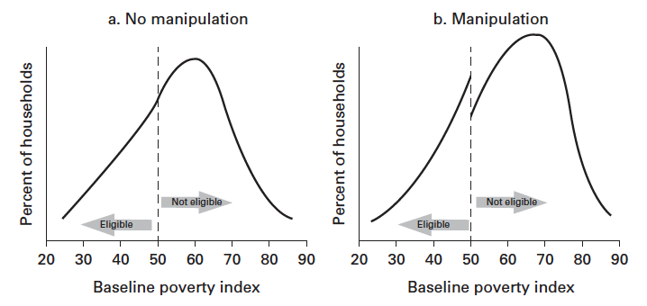
First, the threshold should not be perfectly manipulatable. In order words, the method accommodates some manipulation in case some individuals play around to increase their chances to be included (or excluded) from some intervention. There are different ways of checking the plausibility of this assumption, but perhaps the most used one by applied researchers is the McCrary Density Test. This test check whether there is indication of perfect manipulation of the assignment variable by looking for discontinuities in its density function around the cutoff point.
Second, individuals close to the cutoff point should be very similar, on average, in observed and unobserved characteristics. In the RD framework, this means that the distribution of the observed and unobserved variables should be continuous around the threshold. Even though researchers can check similarity between observed covariates, the similarity between unobserved characteristics has to be assumed. This is considered a plausible assumption to make for individuals very close to the cutoff point, that is, for a relatively narrow window.
Finally, unlike the instrumental variable framework, the RD design does not require the exclusion restriction as the assignment variable (also called running variable or forcing variable) can be directly correlated with the outcome variable (see Lee and Lemieux 2010). The identification strategy in RD design framework requires that conditional on the assignment variable, participation in a program or intervention is exogeneous. This is very similar to the conditional independency assumption, but because of the discontinuity, the assumption is required for individuals lying each side of the threshold.
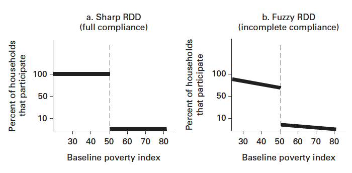
In practice, the assignment rule can be deterministic or probabilistic (see Hahn et al. 2001). If deterministic, the design is called Sharp as the assignment rule defines treatment status with probabilities 0 or 1. If probabilistic, the design is called Fuzzy as the assignment rule defines ‘eligibility’ status rather than ‘treatment’ status. What could cause the fuzziness? Imperfect compliance with some law/rule, imperfect implementation that could end up treating some control units, spillover effects, or some manipulation of the forcing variable could lead to a fuzzy RD design. Thus, the estimates of the causal effect under the fuzzy design require more assumptions than under the sharp design, but are weaker than any IV approach.
The key assumption of a fuzzy design is that without the assignment rule some of those who take up the treatment would not participate in the programme (for similarities between IV and RDD approaches, see Imbens and Lemieux 2008 and van der Klaauw 2008). The forcing variable acts as a nudge. The subgroup that participates in a programme due to the selection rule is called compliers (see e.g. Angrist and Imbens 1994, and Imbens, Angrist, and Rubin 1996). Thus, under the RDD the treatment effects are estimated only for the group of compliers.
For the sake of illustration, let X be the treatment variable, Z the assignment variable and Y the outcome variable. Under sharp design, the treatment variable X is a deterministic function of Z, and equation is discontinuous in some observable values of Z, i.e., ZTemplate:Sub. Defining the observed outcome model as XTemplate:Sub XTemplate:Sup
[[[ Equations missing here ]]]
Although the sharp and fuzzy estimators identify only the local average treatment effect, i.e., the treatment effect for the individuals close to the cut-off, Hahn et al. (2001) note that this method has many advantages compared to other quasi-experimental approaches in that it does not depend on functional form assumptions when estimates can be obtained with narrow bandwidths and does not require identifying instruments or the set of variables that affect the selection rule for a particular programme (or treatment).
That said, the most recent advances in the RDD literature suggest that it is not very accurate to interpret a discontinuity design as a local experiment. To be considered ‘as good as a local experiment for the units close enough to the cutoff point’, one should have to use a very narrow bandwidth and drop the assignment variable (or a function of it) from the regression equation. For more details on this point see Cattaneo et al. (here and here).
Empirical Challenges: Bandwidth Size, Structural Form, and Falsification Tests
The estimation of the treatment effects can be performed parametrically as follows:
[[[ Equations missing here ]]]
where y_i is the outcome of interest of individual i, X_i is an indicator function that takes the value of 1 for individuals assigned to the treatment and 0 otherwise, Z_i is the assignment variable that defines an observable clear cutoff point, and h(Z_i ) is a flexible function in Z. The identification strategy hinges on the exogeneity of Z at the threshold. It is standard to center the assignment variable at the cutoff point. In this case, one would use h(Z_i-Z_0 ) instead with Z_0 being he cutoff. With that assumption, the parameter of interest, δ, provides the treatment effect estimate. In the case of a sharp design with perfect compliance, the parameter δ identifies the average treatment effect on the treated (ATT). In the case of a fuzzy design, δ corresponds to the intent-to-treat effects – i.e. the effect of the eligibility rather than the treatment itself on the outcomes of interest. As discussed above, theThe LATE can be estimated using an IV approach. This could be done as follows:
[[[ Equations missing here ]]]
where P_i is a dummy variable that identify actual participation of individual i in the program/intervention. Notice that with a parametric specification the researcher should specify h(Z_i ) the same way in both regressions (Imbens and Lemieux 2008).
Despite the natural appeal of parametric method such as the one just outlined, this method has some direct practical implications. First, the right functional form of h(Z_i ) is never known. Researchers are thus encouraged to fit the model with different specifications of h(Z_i ) (Lee and Lemieux 2010), particularly when have to consider data farther away from the cutoff point to have enough statistical power. (For those interested in some fresh discussion on power calculation for RD design, please see these links here, here and here).
Although some authors test sensitivity of results using high order polynomials, there is some recent discussion arguing against the use of high order polynomials given that they assign too much weight to observations away of the cutoff point (Imbens and Gelman 2014).
In practice, the size of the window (usually referred to in this literature as bandwidth size) depends on data availability (see discussion below). Ideally, one would like to have enough sample to run the regressions using information very close to the cutoff. The main advantage of using a very narrow bandwidth is that the functional form h(Z_i ) becomes much less of a worry and treatment effects can be obtained with parametric regression using a linear or piecewise linear specification of the assignment variable (see Lee and Lemieux 2010 for this point).
Falsification (or placebo) tests are really important when using RD design as identification strategy. The researcher needs to convince the reader (and referees!) that the discontinuity been exploited to inform causal impacts of an intervention was very much likely caused by the assignment rule to the intervention. In practice, researchers use fake cutoffs or different cohorts to run those tests. Examples can be seen here, here, and here.
Another way of estimating treatment effects with RD design is via non-parametric methods. In fact, the use of non-parametric methods has been growing in the last few years, at least to check robustness of estimates obtained parametrically. This might be partially explained by the increasing number of available STATA commands (if you want to know more about STATA commands for RDD, please using this here) but perhaps more importantly due to some attractive properties of the method compared to parametric ones (see e.g. Imbens and Gelman 2014 for this point).
The use of non-parametric methods does not come without costs. There are still many decisions left to the researcher such as which kernel function to use, which algorithm to use for selection of optimal bandwidth size, and whether to use local linear or any other specification (Imbens and Gelman 2014 suggest the use of local linear and at most local quadratic polynomials).
For those interested in knowing more RD design and its recent ramifications, check this practical introduction (link here). For more advanced stuff, check this e-book.
Back to Parent
This article is part of the topic Impact Evaluation Design
Additional Resources
- An introduction and user guide to Regression discontinuity. Lee, David S., and Thomas Lemieuxa. "Regression discontinuity designs in economics." Journal of economic literature 48, no. 2 (2010): 281-355.


