Power Calculations in Stata
Power calculations indicate the minimum sample size needed to provide precise estimates of the program impact; they can also be used to compute power and minimum detectable effect size. Researchers should conduct power calculations during research design to determine sample size, power, and/or MDES, all of which play critical roles in informing data collection planning, budget, timeline, accuracy, and precision. This page presents different options of Stata commands for power calculations and discusses the advantages and disadvantages associated with each.
Read First
- Optimal Design provides helpful visualizations for power calculations that may aid understanding of power calculations in Stata.
- Stata is better than Optimal Design for reproducible research purposes, as the power calculations are codified in a do file.
- To install the commands covered in this page, search
findit, followed by the command name. Then find the most recent update of the command and install it. For more information on each command, typehelp, followed by the command name. Note thatpoweris Stata’s built-in program for sample size calculations and does not need to be installed. - For more information on the key parameters of power calculations, see Sample Size and Power Calculations.
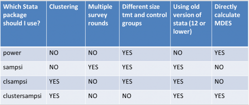
- The below table outlines the capabilities of four Stata commands for power calculations. More detailed descriptions follow.
power
power is a built-in program and Stata’s newest update to power calculations. It was introduced with Stata13 as a replacement to sampsi. It is best used for simple randomizations with no clustering.
Advantages
- Offers more flexibility of input/output choices
- Generates better outputs including more information and a graph option
- Automatically saves output to a file
- Can compute the sample size of control group given a treatment group size (or vice versa)
- Directly calculates MDES
Disadvantages
- No straightforward way to control for repeated measures
- Allows for treatment and control groups of different sizes
Useful Options
power onemean: assumes equal means in treatment and control- Sample size
n(): sample sizen1(): control group sizen2(): treatment group sizenratio: ratio of n1/n2. Its default is 1. It is not necessary to specify this if you specifyn1andn2
tableoutputs results in a table formatsaving(filename, [replace])saves results in a .dta format
sampsi
sampsi is no longer an officially supported Stata package. It has been replaced by power. However, it continues to work. By default, the command computes sample size. To compute power, specify n1 or n2. To compare means (not proportions), specify sd1() or sd2(). For repeated measures, sd1() or sd2() must be specified. Note that sampsi defaults to 90% power.
Advantages
- Works with Stata13 or earlier
- Allows repeated measures (multiple follow-ups)
Disadvantages
- Does not allow clustering
- Requires user to impute MDES
Useful Options
onesample: assumes equal means in treatment and control- Sample size
n1(): size of treatment groupn2(): size of control groupratio(): n1/n2, default is 1
- Repeated measures
pre: number of baseline measurementspost: number of follow-up measurementsr0(): correlation between baseline measures (default r0 = r1)r1(): correlation between follow-up measuresr01(): correlation between baseline and follow-up
method(): options includepost,change,anova, orall. The default isall.sampclusis an add-on tosampsithat allows for clustering. It must be directly preceded bysampsicommand. For example, the following code correct sample size and computes the number of clusters from a t-test. It then adjusts this sample size calculation for 10 observations per cluster and an ICC of 0.2:
sampsi 200 185, alpha(.01) power(.8) sd(30)
sampclus, obsclus(10) rho(.2)
Computing MDES with sampsi
To compute MDES with sampsi, use a guess-and-check method. The difference between baseline and hypothesized mean is MDES. Compute power, using different hypothesized means, aiming for power = 0.8.
clsampsi
Advantages
- Allows for clustering
Disadvantages
- Requires user to impute MDES
- Does not allow for repeated measures
- Does not allow for baseline correlation
Useful options
m(): cluster size in treatment and control, assuming equal cluster size in each group. If the treatment and control cluster sizes differ, usem1()andm2()for the control and treatment cluster sizes, respectively.k(): number of clusters in treatment and control, assuming equal number of clusters in each group. If the number of clusters differs between treatment and control, usek1()andk2()for the control and treatment cluster numbers, respectively.sd(): standard deviation, assuming it is equal between the treatment and control groups. If the treatment and control standard deviation differs, usesd1()andsd2(#)for the control and treatment standard deviations, respectively.rho(#): ICC assuming it is equal between the treatment and control groups. Alternatively, userho1()andrho2().sampsidetermines the power of means (or proportion) comparison using the standardsampsicommandvarm(#): cluster size variation, assuming it is the same between the treatment and control groups. This only affects the power if it is larger thanm()andrho()>0.
clustersampsi
Advantages
- Allows for clustering
- Allows for baseline correlations
- Directly calculates MDES
Disadvantages
- Doesn’t allow for different sized treatment / control groups
- Doesn’t allow for repeated measures
Useful options
detectabledifferencecalculates MDES- Alternative options:
power,samplesize - to use detectable difference, specify
m,k,mu1
- Alternative options:
rho(): ICCk(): number of clusters in each armm()average cluster sizesize_cv(): coefficient of variation of cluster sizes (default is 0). Can be any number greater than 1.mu1()andmu2(): mean for treatment and control, respectivelysd1()andsd2(): mean for treatment and control, respectivelybase_correlcorrelation between baseline measurements – or other predictive covariates – and outcome
Back to Parent
This article is part of the topic Sampling & Power Calculations
Additional Resources
- DIME Analytics guidelines on survey sampling and power calculations 1 and 2
- Batistatou et al.’s Sample size and power calculations for trials and quasi-experimental studies with clustering, which focuses on applications of
clsampsi - Bharti’s Standalone use of STATA for analysis of cluster randomized controlled trials
- Berk Ozler’s Power Calculations: What software should I use? via the Development Impact blog
- Andrew Gelman’s Why it makes sense to revisit power calculations after data has been collected
- JPAL’s The Danger of Underpowered Evaluations

